A synthetic asset has been trading for 10 years. You are given the complete daily price history. A new simulation will now run for exactly 365 days, starting at $10,000.
The asset will be generated in exactly the same manner as it was historically. Your task is to infer the asset's price dynamics from the historical data, then allocate across the available instruments to maximise expected profit.
Key Details
All options are European and held to expiry (day 365).
Options are exercised automatically at expiry.
Risk-free rate = 0%.
There is no margin requirement — you may sell options freely.
You have a portfolio of $1,000,000.
Allocation is specified as % of portfolio:
Positive % = buy that instrument (spend that % of portfolio at the ask)
Negative % = sell that instrument (receive that % of portfolio at the bid)
Total gross exposure (sum of absolute values of all allocations) must not exceed 200%.
The asset price starts at exactly $10,000 each simulation.
Infinite liquidity is assumed at the stated bid/ask prices. You need not worry about how many options are available.
The asset started at $10,000 on day 0. Use this data to characterise the asset's dynamics.
Your Submission
Enter your allocation for each instrument as a percentage of your $1,000,000 portfolio using the form below.
Sign convention:
Positive = buy at the ask price
Negative = sell at the bid price
e.g. +10.0 on Call 30,000→spend100,000 buying calls at $396.56 each
e.g. -5.0 on Put 60,000→sell50,000 worth of puts at $47,043.45 each
Scoring
All submissions are evaluated on the same 10,000 simulated price paths. The paths are generated from a random seed drawn at scoring time — not disclosed beforehand.
Each path:
The asset evolves for 365 days from $10,000 under the true DGP.
All options are settled at fair value on day 365.
Your PnL is computed as: sum of option payoffs minus sum of premiums paid (or plus premiums received for shorts).
Score = average PnL across all 10,000 paths, measured in $.
Higher is better. You can lose money. Every participant faces the same price realisations, so rankings reflect analytical skill rather than Monte Carlo variance.
Notes and Cautions
The market prices may or may not reflect the true fair values of the instruments. Determining whether and where mispricing exists is the core of this problem.
A score of $0 is achievable trivially by submitting all zeros.
Positive returns require identifying mispriced instruments and sizing positions accordingly.
Positions in very expensive options (e.g. deep ITM puts) require large allocations to generate meaningful position sizes — be careful about what you are paying per unit.
Background reading
European options — options that can only be exercised at expiry.
Black-Scholes model — the standard model for pricing European options under log-normal assumptions.
Log-normal distribution — the return distribution assumed by Black-Scholes. Real assets often have heavier tails.
This problem gives you 10 years of daily price data for a synthetic asset and asks you to allocate across the underlying and a set of European options. The key is figuring out how the asset actually moves, then comparing your model's fair values to the market prices to find mispriced instruments.
Step 1: Identify the data-generating process
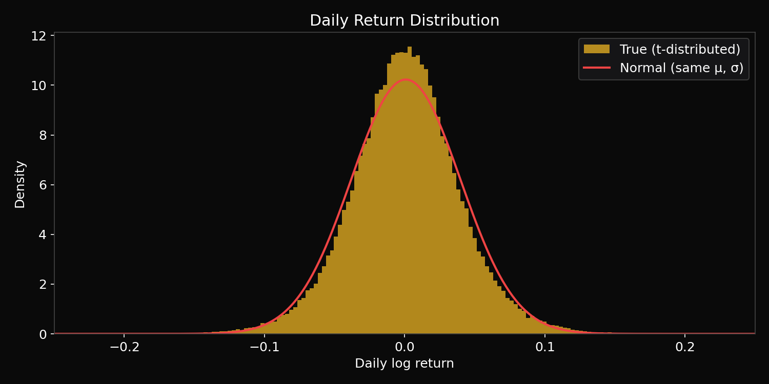
The historical data contains 3,650 daily observations. Plotting daily log returns reveals two things:
Positive drift — the asset trends upward over time.
Fat tails — extreme daily moves occur more often than a normal distribution would predict. The distribution is leptokurtic (peaked centre, heavy tails).
The red curve shows a normal distribution with the same mean and standard deviation. The true returns are sharply peaked in the centre and have fatter tails — a classic signature of Student's t-distributed innovations.
Fitting a t-distribution to the standardised returns via maximum likelihood gives approximately:
Parameter
Fitted value
μ (daily drift)
~0.0008
σ (daily vol)
~0.039
ν (degrees of freedom)
~8
The degrees of freedom parameter is the important one. At ν = 8, tail events are substantially more likely than under normality. A 4σ move happens roughly 5x more often than a normal model predicts.
Step 2: Simulate terminal prices
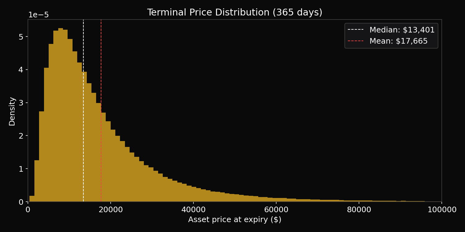
With the fitted parameters, you can Monte Carlo the terminal price distribution after 365 days:
The distribution is right-skewed with a long upper tail. The mean ($17,700) is well above the median ($13,400) because rare large upward moves pull the average up. This matters for option pricing: the expected payoff of a call option depends heavily on the right tail.
Step 3: Price the options and find mispricing
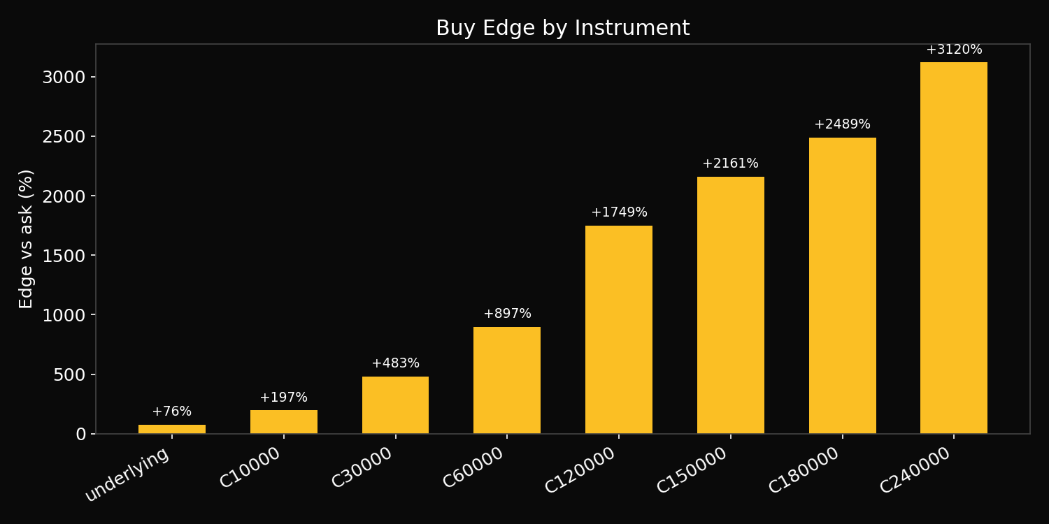
The market prices in this problem were generated using a model that underestimates both the drift and the tail thickness of the true DGP. This creates systematic mispricing:
Every call option is underpriced relative to the true DGP. The percentage edge grows with strike: ATM calls are underpriced by ~200%, while the far OTM call at $240k is underpriced by over 3000%. This happens because the market's thinner-tailed model assigns near-zero probability to the asset reaching $240k, but the true fat-tailed process gets there often enough to make the option worth far more than $0.08.
Percentage edge is not the same thing as contest-optimal allocation. There are two extra constraints:
Positions are sized by dollar allocation, so what matters is expected PnL per dollar allocated.
The final score is estimated on 10,000 shared Monte Carlo paths, so extremely rare payoffs have real finite-sample risk.
In a very large simulation, the $240k call has the highest true expected PnL per dollar because the rare paths where it pays are enormous:
Instrument
Large-sample expected PnL per 100% allocation
call_240000
$37.3m
call_180000
$22.8m
call_150000
$19.2m
call_120000
$15.9m
call_60000
$8.8m
call_30000
$4.8m
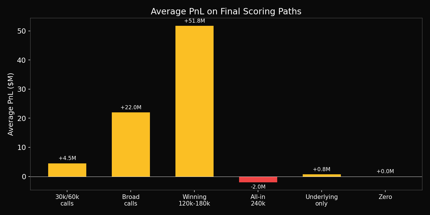
That does not mean going all-in on the $240k call is robust. Its payoff depends on very few paths. On the final shared scoring paths, no simulated terminal price finished above $240k, so a 200% allocation to call_240000 lost the full $2m premium. The strongest realised single-instrument allocations on those paths were instead the $150k, $120k, and $180k calls.
On the put side, the ATM put ($10k strike) is overpriced — the market charges ~$2,990 for downside protection that is worth only ~$1,200 under the true model. Selling it is profitable in expectation. Deeper OTM puts are roughly fairly priced or underpriced on the ask side, making them poor buys.
Step 4: Size positions
The scoring rule is average PnL, which is linear in position size. This means you should concentrate on the highest-edge instruments and size up to the 200% gross exposure limit.
Buying OTM calls generates the highest average PnL. The mistake is stopping too close to the money. The 30k and 60k calls are genuinely good trades, but they are not the most capital-efficient ones:
The 30k and 60k calls finish in-the-money more often, but their payoffs are much less convex.
The 120k-180k calls are far enough out that they benefit heavily from the fat right tail, but not so far out that the score becomes a pure lottery on one or two paths.
The 240k call has the highest large-sample EV, but in a 10,000-path scoring run it can easily receive zero hits. That is exactly what happened in the final scoring run.
The relevant terminal-price hit counts on the final scoring paths were:
Terminal price threshold
Paths above threshold
$60k
201 / 10,000
$120k
19 / 10,000
$150k
11 / 10,000
$180k
3 / 10,000
$240k
0 / 10,000
So the best contest allocation balanced tail exposure and hit frequency. It moved past the 60k call, where much of the convexity had already been spent, but stopped short of putting everything into the 240k strike.
The winning allocation used the full 200% gross exposure limit:
Instrument
Allocation
call_120000
+100%
call_150000
+70%
call_180000
+30%
On the final shared scoring paths this produced an expected PnL of about $51.8m. A more diversified "buy lots of calls" solution still scored well, but spreading allocation into 30k/60k calls left a lot of expected value on the table, while concentrating entirely in 240k exposed the portfolio to too much finite-sample tail risk.
Key concepts
Fat tails and option pricing: Black-Scholes assumes log-normal returns (Gaussian innovations). When the true process has fatter tails, Black-Scholes underprices OTM options because it underestimates the probability of large moves. This is why volatility smiles exist in real markets — OTM options trade above their Black-Scholes values because traders know tails are fat (Cont 2001).
Physical vs risk-neutral measure: The market prices here are closer to risk-neutral pricing (discounting the drift), while scoring is under the physical measure (actual drift included). This is an additional source of edge — even if the market correctly modelled the tail shape, it would still underprice calls if it used risk-neutral drift instead of the true positive drift.
MLE for distribution fitting: Maximum likelihood estimation of the t-distribution parameters from historical returns is the standard approach (Bollerslev 1987). The QQ plot of standardised returns against a t-distribution with the fitted ν is a good diagnostic — if the points lie on the 45° line, the fit is good.
What separated good from great
Recognising non-normality. A histogram or QQ plot of returns immediately shows fat tails. Participants who assumed normality (or used Black-Scholes directly) would have underestimated the value of OTM calls.
Fitting the right model. The t-distribution with ~8 degrees of freedom captures the tail behaviour well. Fitting it via MLE rather than eyeballing gives more accurate option prices.
Understanding the edge direction. All calls are underpriced, all deep puts are roughly fair. The profitable trade is buying calls, not selling puts. Participants who sold puts (a common instinct — "collect premium") earned less than those who bought calls.
Moving far enough out the call chain. The 30k/60k calls were profitable but not optimal: they had less convex exposure to the fat right tail than the 120k-180k calls.
Not moving too far out. The 240k call had the highest large-sample expected value, but its payoff was too sparse for a 10,000-path contest score. It received zero hits on the final scoring paths.
Sizing aggressively on the sweet spot. The scoring rule rewards expected PnL, not risk-adjusted returns. Concentrating on the best OTM calls and using the full 200% gross limit maximises the score.